📌 Introduction
Linear regression is the process of finding a line in a graph that best fits the data. It is a type of supervised learning, meaning it uses labeled data (datasets that already include the correct answers). It’s one of the first things that people learn when starting their machine learning journey.
🧠 The Big Idea
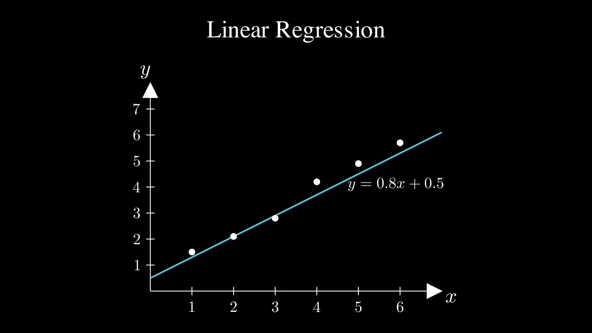
Just as I mentioned above, you only have to think of linear regression as fitting the best line to the data! You probably know that the equation of a line is:
$y = wx + b$
In this equation, $w$ is the slope (how steep the line is), and $b$ is the intercept (where the line crosses the y-axis). So to fit the line, you would have to change the $w$ and $b$ values.
📊 What does It Actually Do?
By fitting a line which is close to all data, we would be able to predict the $y$ values of any input $x$. Let’s use house prices as an example 🏠 (it’s one of the most common examples).
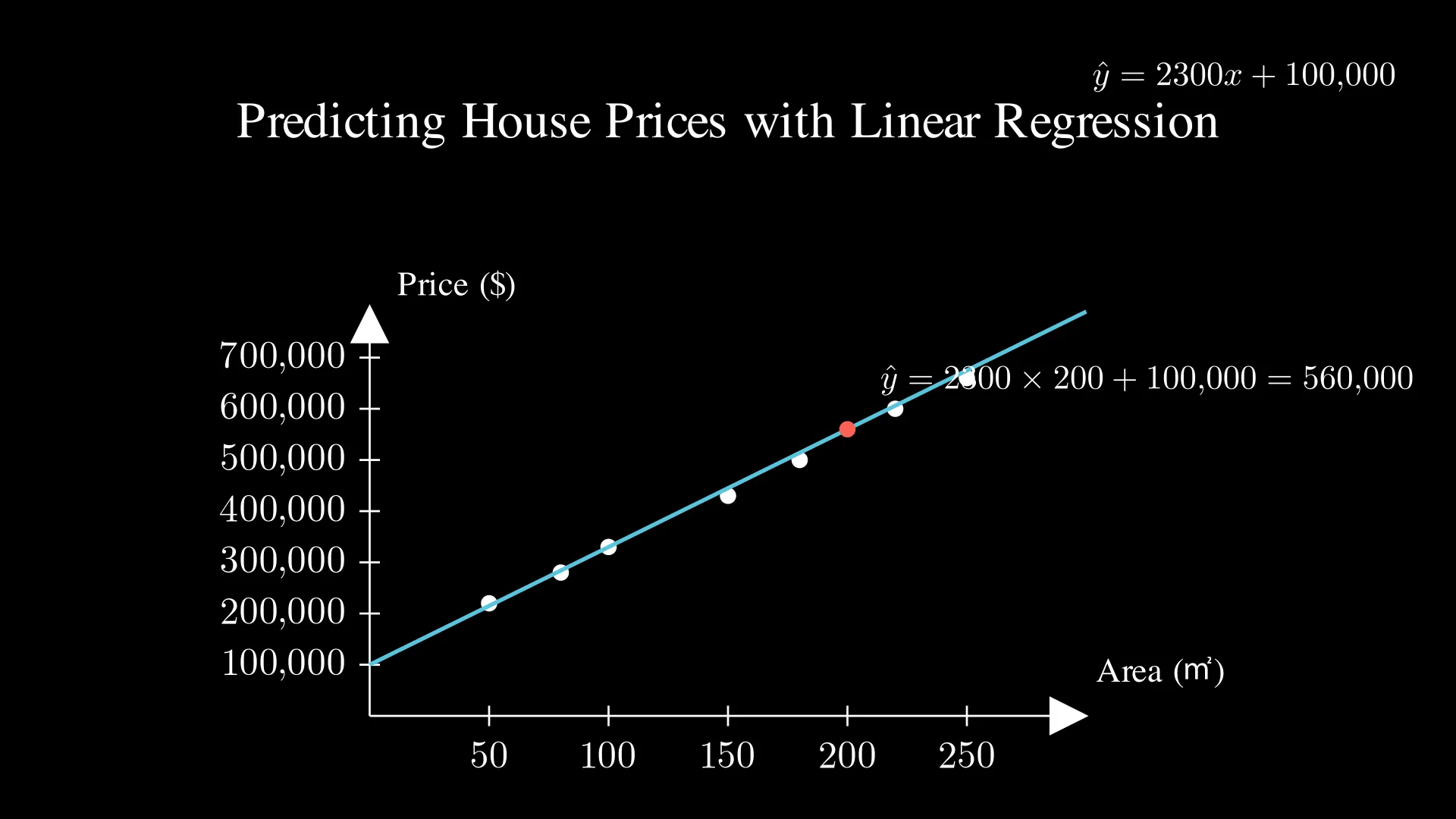
In this graph, the white dots represent the data (e.g., a 180 m² house costing 500k), and by linear regression, we can find the blue line that best fits the data. Since we have this line, we can now predict house prices by finding the corresponding values of the line. For example, let’s say that we want to predict the price of a 200 m² house. Because the equation of the line is:
$\hat{y} = 2300x + 100,000$
ℹ️ Note:
The symbol $\hat{y}$ (y-hat) is commonly used to denote predicted values in statistics and machine learning. This helps distinguish predicted values ($\hat{y}$) from actual outcomes ($y$) in the training data.
The predicted price of this house would be:
$\hat{y} = 2300 \times 200 + 100,000 = 560,000$
And voila! We’ve just used linear regression to predict house prices 😄
🔍 How Does It Learn?
You now might be curious about how we actually find the best fitting line. And that’s exactly what I’m going to tell you.
Finding the best fitting line is the same as finding the lowest cost. And the cost is measured by a cost function, which measures the performance (cost) of a model. There are many cost functions used for many cases, but I will use Mean Squared Error (MSE) (which is the default for most regression problems) to explain how linear regression learns.
This is the formula for Mean Squared Error:
$J(\vec{w}, b) = \frac{1}{m} \sum_{i=1}^{m} (y_i - \hat{y}_i)^2$
The cost increases if the difference between the predictions ($\hat{y}$) and the actual values ($y$) are larger, and the cost decreases if the predictions ($\hat{y}$) are close to the actual values ($y$).
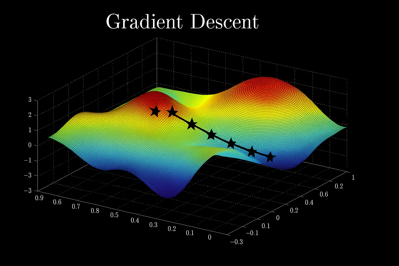
We now know that we can use the cost function to evaluate the performance of the model. Now it’s time for me to tell you about gradient descent, which is a method that allows us to minimize the cost (and eventually allow us to find the best parameters - such as the slope and the intercept of our line).
Suppose you’re on a hill, and say you have to go down the hill as quickly (efficiently) as possible because you really have to use the bathroom. However, there’s a problem: it’s super cloudy, and you can only see things that are close to you. You’ll probably take the steepest step, right? Because you’ll want to go down quickly. You will repeat the process until you reach the lowest part of the hill. What you’ve just done is similar to what gradient descent does: it takes the steepest step to minimize the cost.
This is the gradient descent formula for linear regression:
repeat {
$w = w - \alpha \dfrac{\partial J}{\partial w}$
$b = b - \alpha \dfrac{\partial J}{\partial b}$
}
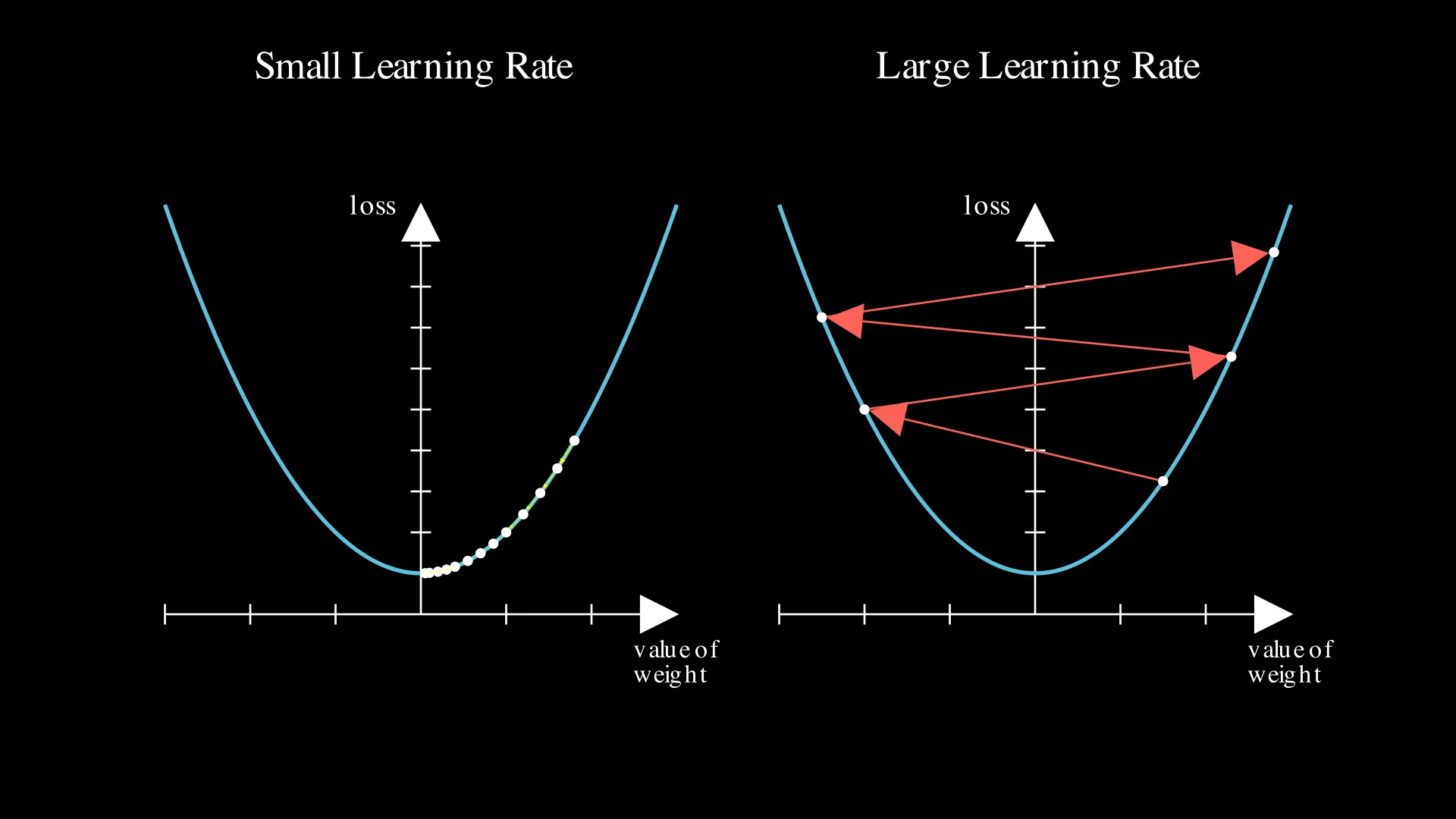
Here, $\dfrac{\partial J}{\partial w}$ and $\dfrac{\partial J}{\partial b}$ are the gradients. The gradients allow us to take the steepest step. $\alpha$ (alpha) is called the learning rate. You could think of this as the ‘size’ of the steps. If the learning rate is too small, linear regression learns slower, as the steps are small. However, if the learning rate is too big, it could diverge and never be able to minimize the cost. The image below visualizes what happens when the learning rate is too small or big:
🛠️ Building It From Scratch
Now that you know how linear regression learns, let’s build it from scratch!
We will use the diabetes dataset from scikit-learn. Let’s start off by loading the data:
from sklearn.datasets import load_diabetes
from sklearn.preprocessing import StandardScaler
import numpy as np

data = load_diabetes()
X = data.data   # shape: (442, 10)
y = data.target # shape: (442,)

# Standardize features (mean=0, std=1)
scaler = StandardScaler()
X = scaler.fit_transform(X)

X = X.T           # shape: (10, 442)
y = y.reshape(-1) # shape: (442,)
Let’s now build the linear regression model:
def initialize_parameters(dim):
    w = np.zeros((dim, 1))
    b = 0.0

    return w, b

def propagate(w, b, X, y):
    m = X.shape[1]

    # Forward propagation
    Z = np.dot(w.T, X) + b
    y_hat = Z

    # Mean squared error (we use 1/2 to simplify gradients)
    cost = (1 / (2* m)) * np.sum((y - y_hat) ** 2)

    # Backward propagation
    dZ = y_hat - y
    dw = (1 / m) * np.dot(X, dZ.T)
    db = (1 / m) * np.sum(dZ)

    grads = {
        "dw": dw,
        "db": db
    }

    return grads, cost

def optimize(w, b, X, y, num_iterations=5000, learning_rate=0.01):
    for iteration in range(num_iterations):
        # Propagation
        grads, cost = propagate(w, b, X, y)

        # Retrieve gradients
        dw = grads["dw"]
        db = grads["db"]

        # Update parameters (gradient descent)
        w = w - learning_rate * dw
        b = b - learning_rate * db

        # Print cost every 1000 iterations
        if iteration % 1000 == 0:
            print(f"Iteration={iteration}: cost={cost:.6f}")

    parameters = {
        "w": w,
        "b": b
    }

    return parameters, cost

def predict(w, b, X):
    y_pred = np.dot(w.T, X) + b
    return y_pred

def model(X, y, num_iterations=5000, learning_rate=0.01):
    w, b = initialize_parameters(X.shape[0])
    parameters, cost = optimize(w, b, X, y, num_iterations, learning_rate)

    w = parameters["w"]
    b = parameters["b"]

    y_pred = predict(w, b, X)

    # Print accuracy
    print("Mean Squared Error: {:.6f}".format(cost * 2))

    d = {"y_pred": y_pred,
         "w" : w,
         "b" : b,
         "learning_rate" : learning_rate,
         "num_iterations": num_iterations}

    return d
Time to train the model!
linear_regression_model = model(X, y)
Output:
Iteration=0: cost=14537.240950
Iteration=1000: cost=1439.357018
Iteration=2000: cost=1437.811167
Iteration=3000: cost=1436.547908
Iteration=4000: cost=1435.491481
Mean Squared Error: 2869.207583
With this dataset, MSE of about 2900 with linear regression is considered successful — meaning that we’ve just built a working linear regression model!
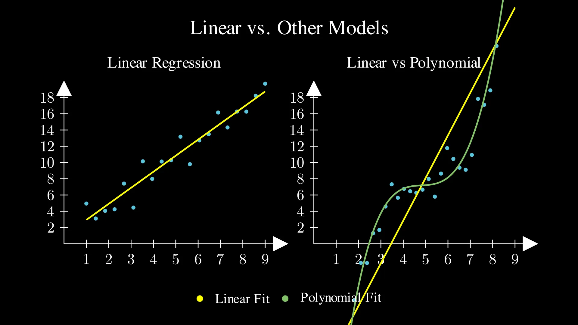
📚 Linear vs. Other Models
Linear regression is simply fitting a line to the data. So it works best when the data is linear. However, what if the data isn’t linear? In that case, other models (such as polynomial regression) work better. The image below shows when linear regression works well and doesn’t work well:
If you want to explore what comes next, the scikit-learn linear models guide is a great place to start with.
✅ Summary
In this blog post, we’ve looked at how linear regression works, when we use it, and the core concepts behind it. It’s a great starting point in machine learning as gradient descent and cost functions are actually very important in many machine learning models.
In the next blog post, we’ll explore logistic regression, which is another important model in machine learning. See you then!