📌 Introduction

Previously, we’ve learned that linear regression was fitting the best line through data. Logistic regression fits an S-shaped curve (sigmoid function) to the data. Logistic regression is also a type of supervised learning (has labeled data), and while linear regression is a regression model which predicts continuous values for its output, logistic regression is a classification model (although it’s called logistic ‘regression’), which can only have two possible outputs: 0 and 1. This model is used to find out yes or no questions. Such as spam detection (is this a spam or not?), medical diagnosis (does this person have a disease or not?), and fraud detection (is this a fraudulent transaction or not?).

🧠 The Big Idea

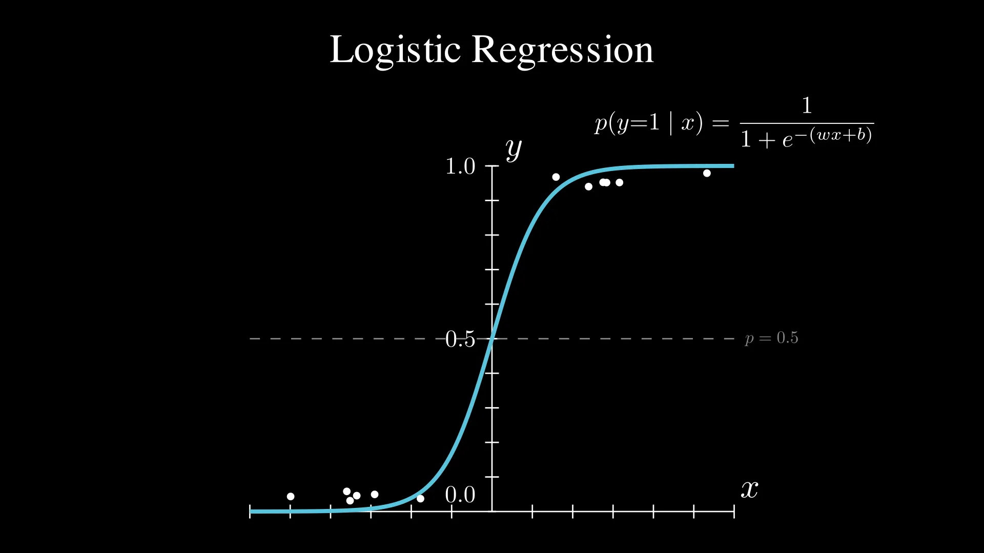
Instead of predicting continuous values like linear regression, logistic regression predicts probabilities. As I mentioned above, you predict the probabilities through the S-shaped curve, also called the sigmoid function or the logistic function. The equation for the sigmoid function is:
$\sigma(z) = \frac{1}{1 + e^{-z}}$
where
$z = wx + b$
From the graph above, we could notice that as the input value $x$ increases, the predicted probability increases as well. Through the sigmoid function, we could separate data.

🧩 How It Works

Logistic regression works as follows:

1. Take input features: in this example, let’s create an algorithm that predicts if a student will pass their test based on study hours.
2. Compute the weighted sum: $z = w x + b$ (similar to linear regression).
3. Apply the sigmoid function: $\hat{y} = \sigma(z) = \dfrac{1}{1 + e^{-z}}$ (this will give us a probability between 0 and 1)
4. Make a prediction:
   • If $\hat{y} \geq 0.5$, predict Class 1 (e.g., the student passes).
   • If $\hat{y} < 0.5$, predict Class 0 (e.g., the student fails).

ℹ️ Note:

In $\hat{y} \geq 0.5$ and $\hat{y} < 0.5$, the value $0.5$ is called the decision boundary. The decision boundary is usually 0.5, but it could be a different value based on the problem. For example, if we are creating a disease detection algorithm, and this algorithm will be used to flag ‘potential’ diseases, we could lower the decision boundary to let’s say 0.3.

🔍 How Does It Learn?

We’ve learned that we need cost functions in order to use gradient descent to find the best fitting graph in the data (this is explained in the previous blog). However, if we use the same cost function as linear regression (MSE) for logistic regression, we get a cost function as below:

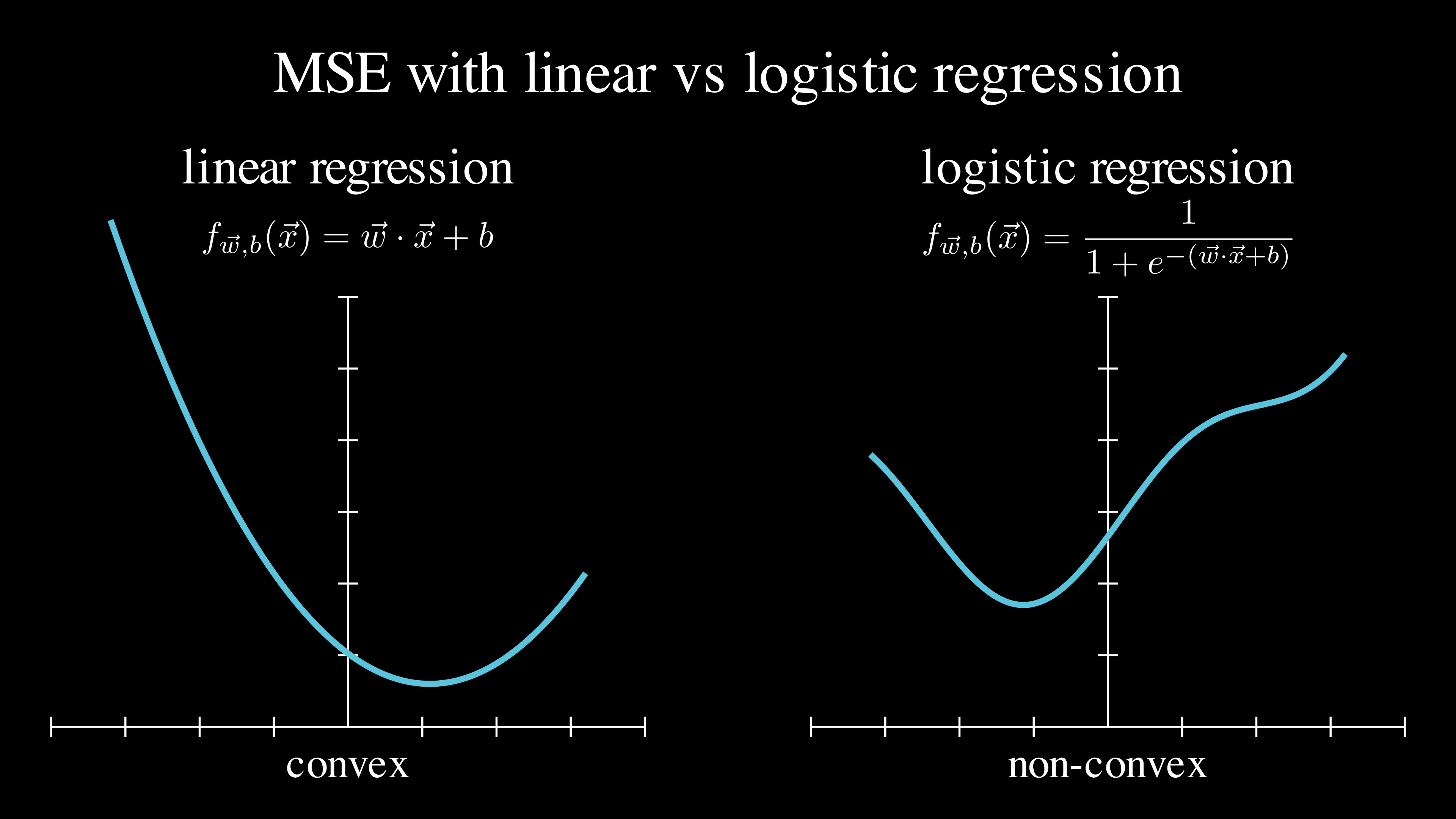
As you could see, while the cost function plot for linear regression is a smooth convex, the cost function plot for logistic regression is a wiggly non-convex. This makes it hard to reach the global minimum since there are many local minima where gradient descent can get stuck. Instead, we use a different cost function: binary cross-entropy (also called Log Loss)! This is the formula of binary cross-entropy:

\(J(w, b) = -\frac{1}{m} \sum_{i=1}^{m} \Big[ y^{(i)} \log\big(\hat{y}^{(i)}\big) + \big(1 - y^{(i)}\big) \log\big(1 - \hat{y}^{(i)}\big) \Big]\)

It looks very complicated, right? Let’s dive in to the specific details so that you will eventually understand what’s happening in this formula.
First, you have to understand the difference between a cost and a loss. The main difference is that loss is for only one example and cost is for all the examples (the sum of all the loss). The formula for binary cross-entropy derives from this formula for calculating a single loss:

\(L\left(f_{\vec{w},b}\left(\vec{x}^{(i)}\right),\, y^{(i)}\right) = \begin{cases} -\log\left(f_{\vec{w},b}\left(\vec{x}^{(i)}\right)\right) & \text{if } y^{(i)} = 1 \\\\ -\log\left(1 - f_{\vec{w},b}\left(\vec{x}^{(i)}\right)\right) & \text{if } y^{(i)} = 0 \end{cases}\)

This is the plot for $-\log\left(f\right)$ and $-\log\left(1 - f\right)$:

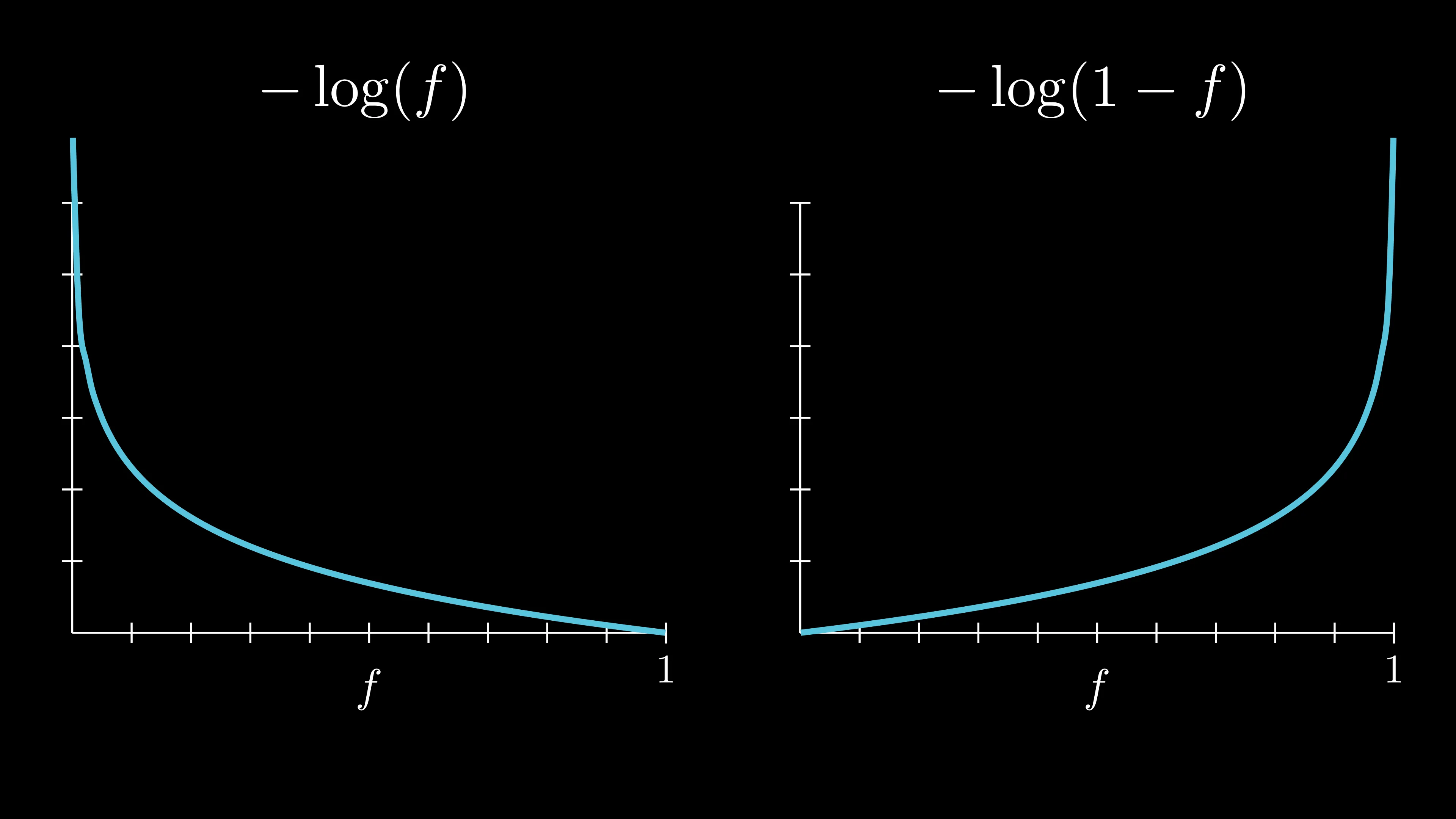
As you can see, in $-\log\left(f\right)$, as the value of $f$ get’s closer to 0, the loss increases. That’s why we use this function if $y^{(i)} = 1$ (because we want to have high loss when our prediction is far from the actual ground truth). Similarly, we use $-\log\left(1 - f\right)$ if $y^{(i)} = 0$ because we want to have low loss when the prediction is close to 0 and have high loss when it’s close to 1. The formula for calculating a single loss can be writen in a more compact form like this:

\(L\big(f_{\vec w, b}(\vec x^{(i)}), y^{(i)}\big) = - \Big[ y^{(i)} \log \hat y^{(i)} + (1 - y^{(i)}) \log \big(1 - \hat y^{(i)}\big) \Big]\)

ℹ️ Note:

When $y^{(i)} = 1$, $\big(1-y^{(i)}\big) \log\big(1 - f_{\vec{w},b}(\vec{x}^{(i)})\big)$ cancels out, leaving us with $- y^{(i)} \log\big(f_{\vec{w},b}(\vec{x}^{(i)})\big)$; and similarly when $y^{(i)} = 0$.

Finally, if we add all the individual losses to find out the cost, we get this formula (same as the one above):

\(J(w, b) = -\frac{1}{m} \sum_{i=1}^{m} \Big[ y^{(i)} \log\big(\hat{y}^{(i)}\big) + \big(1 - y^{(i)}\big) \log\big(1 - \hat{y}^{(i)}\big) \Big]\)

Since we have the cost function, we can now use gradient descent to minimize the cost (I’m thinking about writing a blog post about explaining the details of gradient descent - like backpropagation - in the future) and find the best fitting S-shaped curve.

🛠️ Building It From Scratch

Now, I’ll show you how to build logistic regression from scratch.

ℹ️ Note:

The following code includes some other concepts, such as standardization and preventing overflow, which we haven’t covered in this blog post. However, I hope you would get some general sense of how it is implemented in code.

Where going to use a real-life dataset: the breast cancer dataset. Let’s first load the dataset and shape it so that it would be easier to handle:

import numpy as np
from sklearn.datasets import load_breast_cancer
from sklearn.preprocessing import StandardScaler

data = load_breast_cancer()
X = data.data   # shape: (569, 30)
y = data.target # shape: (569,)

# Standardize features (mean=0, std=1)
scaler = StandardScaler()
X = scaler.fit_transform(X)

X = X.T           # shape: (30, 569)
y = y.reshape(-1) # shape: (569,)

Now that the data is ready, let’s define the logistic regression model:

def sigmoid(z):
    z = np.clip(z, -500, 500) # prevent overflow
    return 1 / (1 + np.exp(- z))

def initialize_parameters(dim):
    w = np.zeros((dim, 1))
    b = 0.0

    return w, b

def propagate(w, b, X, y):
    m = X.shape[1]
    
    # Forward propagation
    Z = np.dot(w.T, X) + b
    A = sigmoid(Z)

    # Clip A to prevent log(0)
    A = np.clip(A, 1e-10, 1 - 1e-10)

    # Binary cross-entropy
    cost = - (1 / m) * np.sum(y * np.log(A) + (1 - y) * np.log(1 - A))

    # Backward propagation
    dZ = A - y
    dw = (1 / m) * np.dot(X, dZ.T)
    db = (1 / m) * np.sum(dZ)

    grads = {
        "dw": dw,
        "db": db
    }

    return grads, cost

def optimize(w, b, X, y, num_iterations=5000, learning_rate=0.5):
    for iteration in range(num_iterations):
        # Propagation
        grads, cost = propagate(w, b, X, y)
    
        # Retrieve gradients
        dw = grads["dw"]
        db = grads["db"]

        # Update parameters (gradient descent)
        w = w - learning_rate * dw
        b = b - learning_rate * db
        
        # Print cost every 1000 iterations
        if iteration % 1000 == 0:
            print(f"Iteration={iteration}: cost={cost}")

    parameters = {
        "w": w,
        "b": b
    }

    return parameters

def predict(w, b, X):
    A = sigmoid(np.dot(w.T, X) + b)
    # 1 if A > 0.5, 0 if A <= 0.5
    y_pred = (A > 0.5).astype(int)
    return y_pred

def model(X, y, num_iterations=5000, learning_rate=0.5):
    w, b = initialize_parameters(X.shape[0])
    parameters = optimize(w, b, X, y, num_iterations, learning_rate)

    w = parameters["w"]
    b = parameters["b"]

    y_pred = predict(w, b, X)

    # Print accuracy
    print("Accuracy: {} %".format(100 - np.mean(np.abs(y_pred - y)) * 100))

    d = {"y_pred": y_pred, 
         "w" : w, 
         "b" : b,
         "learning_rate" : learning_rate,
         "num_iterations": num_iterations}

    return d

Now’s the fun part, let’s run the model!

logistic_regression_model = model(X, y, num_iterations=10000, learning_rate=0.1)

Output:

Iteration=0: cost=0.6931471805599453
Iteration=1000: cost=0.060577603724407784
Iteration=2000: cost=0.05464065759612664
Iteration=3000: cost=0.05197827952420055
Iteration=4000: cost=0.050354290732159204
Iteration=5000: cost=0.0491906287855795
Iteration=6000: cost=0.0482773149756525
Iteration=7000: cost=0.04752096083469107
Iteration=8000: cost=0.04687285954869561
Iteration=9000: cost=0.04630445974594589
Accuracy: 98.76977152899825 %

There you go! We’ve just built logistic regression from scratch!

📚 Logistic vs. Other Models

I hope that now you can confidently explain the difference: logistic regression predicts probabilities (classification), while linear regression predicts continuous values (regression). However, like linear regression, logistic regression is the simplest form of classification models, so it could struggle with non-linear boundaries (e.g., data that is not linearly separable).

✅ Summary

In this blog post, we’ve learned that logistic regression predicts probabilities and classifies based on a threshold. We’ve also learned that logistic regression uses the sigmoid function, binary cross-entropy, and gradient descent to learn. By learning this model, I believe that you now have a solid foundation for classification problems! See you in the next blog post 😊